Non-normal bivariate distributions with normal marginal distributions

It’s well known that the ratio of two independent standard normal random variables has a Cauchy distribution. Let’s prove it! Suppose our normal random variables are X and Y. The kernel of the density is

We do this change of variables:

By a happy chance the Jacobian of this transformation is constant and so, with a little harmless disregard for the region of integration, we substitute directly into the joint density function and get

By inspection we can see that we’ve got the joint density of a Cauchy random variable C and, conditional on C, an exponential random variable T with rate (1 + C²)/2. (The kernel of the Cauchy density and the rate parameter of the exponential density are shown explicitly in the second line; in the first line they have effectively cancelled out.) Thus we have shown that the ratio of two independent standard normal random variables is indeed Cauchy.

We can do a little more with this result though. It shows how to generate two independent normal random variates from a Cauchy and an Exponential (and one more random bit) via the following recipe. Generate, independently:

• a Cauchy random variable C,
• a Rademacher random variable S (which takes the value +1 with 50% probability and the value -1 with 50% probability), and
• an Exponential random variable (with rate 1) U.

Set

Independent standard normal random variables aren’t too interesting; this recipe is worth considering because it gives us a way to generate something a lot more fun: three distinct (and very pretty) bivariate distributions, each non-normal but with normal marginal distributions. (Of course, there’s a boring brute force way to make such a distribution: pick any non-Gaussian bivariate copula and push the marginal uniform random variables through the normal quantile function. Yawn.) We’ll do this by making two independent copies of each of the three random variables in our recipe; that is, we’ll have C_i, S_i, and U_i for i ∈ {1,2}. Now we use the i = 1 variables and follow the recipe as above,

And then we mix the indices to create two more marginally normal variables that have a complicated dependence relation to the previous set:

So what kind of distributions did we make? Well, we’ve defined four distinct marginally normal random variables which gives rise to six bivariate distributions. The three interesting distributions are those of (W, X), (W, Y), and (V, Y). The other three pairs fail to spark joy: X and Y are independent standard normal by definition; V and W would be too except I didn’t bother to give them different signs so their joint distribution is only defined in the first and third quadrants; and it turns out that the pair (V, X) just has the same bivariate distribution as (V, Y).

Let’s sample some, uh, samples and see what we get.

And here’s the code, ready to go.

“Baroque possibilities” for constructing SEV in sequential trials

I mentioned in my last post that I had thought up some baroque possibilities for candidate SEV functions in sequential trials. I figure it’s worth writing out exactly what I mean by that. Before I begin, though, I will direct readers to the first 26 slides of this slide deck, especially the plot on slide 6.

As discussed in the slide deck, when you’re designing a two-sided confidence interval procedure you have some freedom to decide, for each value of the true parameter, how much probability mass you will put above (literally above if we’re talking about the plot on slide 6) the upper limit and how much you’ll put below the lower limit. The confidence coverage property only constrains the sum of these two chunks of probability mass.

The kinds of inferences for which the SEV function was designed are one-sided, directional inferences — upper-bounding inferences and lower-bounding inferences — so there’s no arbitrariness to SEV with well-behaved models in fixed sample size designs. Sequential designs introduce multiple thresholds at which alpha can be “spent” so even just for a simple one-sided test there is already an element of arbitrariness that must be eliminated by recourse to an alpha-spending function or an expected sample size minimization or some other principle that eats up the degrees of freedom left over after imposing the Type I error constraint. There is likewise arbitrariness in specifying a one-sided confidence procedure for sequential trials — as with two-sided intervals there are multiple boundaries to specify at each possible parameter value and the confidence coverage constraint only ties up one degree of freedom.

In the last post I asserted that the conditional procedure was an exact confidence procedure. Here’s the math. Let q₄(α, μ) and q₁₀₀(α, μ) be the quantile functions of the conditional distributions:

Then the confidence coverage of the conditional procedure is

The conditional procedure had the difficulty that its inferences could contradict the Type I error rate of the design at the first look. However, we can replace the quantile functions with arbitrary functions as long as they satisfy that same equality for all values of μ and this will also define an exact confidence procedure. The question then becomes what principle/set of constraints/optimization objective can be used to specify a unique choice.

This sort of procedure offers very fine control over alpha-spending at each parameter value, control that is not available via the orderings on the sample space discussed in the last post that that treat values at different sample sizes as directly comparable. But the phrasing of the (S-2) criterion really strongly points to that kind of direct comparison of sample space elements, and Figure 4 of the last post shows that this is a non-starter. So, to defend the SEV approach from my critique it will be necessary to: (i) overhaul (S-2) to allow for the sort of fine control available to fully general confidence procedures, (ii) come up with a principle for uniquely identifying one particular procedure as the SEV procedure, ideally a principle that is in line with severity reasoning as it has been expounded by its proponents up to this point — oh, and (iii) satisfy PRESS, let’s not forget that.

The SEV function just plain doesn’t work

Introduction

I had a different follow-up planned for my last post but I made a discovery (see title) that caused me to change course. Previously I had made the rather weak point that the SEV function had some odd properties that I didn’t think made sense for inference. Mayo’s response (on Twitter) was: “The primary purpose of the SEV requirement is to block inference as poorly warranted, & rigged exes have bad distance measures.” In this post I’ll argue that the SEV function has properties that I don’t think anyone can claim make sense for inference, and I’ll draw out the consequences of affirming the severity rationale in spite of its possession of these undesirable properties.

Here I’ll examine the SEV function in the context of a modification of Mayo’s “water plant accident” example. For the picturesque details you can follow the link; I’ll stick with the math. The model is normal with unknown mean μ and a standard deviation of 10. Here we are interested in testing H₀: μ ≤ 150 vs. H₁: μ > 150. Mayo looks at the test based on the mean of 100 samples, which I will call x̅₁₀₀. My modification is this: we’ll check the mean after collecting 4 samples, x̅₄, and reject the null if it’s greater than some threshold; otherwise we’ll collect the remaining 96 samples and test again using x̅₁₀₀ as our statistic. Which threshold? It hardly matters, but let’s say the threshold for rejection of H₀ and cessation of data collection at n = 4 is at x̅₄ = 165, three standard errors from the null. (This “spends” 0.00135 of whatever Type I error rate we’re willing to tolerate. In Mayo’s example the Type I error rate is set to 0.022, corresponding to a threshold at x̅₁₀₀ = 152, two standard errors from the null; in our case, to compensate for the look at n = 4 the threshold at n = 100 increases a very tiny amount — it’s 152.02. Nothing turns on these details.) I’ll also consider what happens when the design is to collect not 96 but 896 additional samples for a total of 900 before the second look.

This is an early stopping design (a.k.a. group sequential design, adaptive design correction); they’re common in clinical trials where it’s desirable to minimize the number of patients in the event that strong evidence has been observed. Is it a “rigged” example? It sure is. The rigging lies in the fact that in clinical trials the “looks” at the data wouldn’t be as early as this — it generally isn’t worth looking when only 1/25 of the second-look sample size has been observed, much less 1/225. By using this schedule I am deliberately amplifying problems for frequentist inference that already exist in a milder form in more typical trial designs. But we’ve been told that SEV’s primary purpose is to block poorly warranted inferences, and the question we should be asking isn’t “is it rigged?” — it’s whether SEV actually does a reasonable job even in, or perhaps especially in, setups that don’t make a lot of sense. It is, if you will, a severe test of severity reasoning. In any event, I think even a weird design like this ought to be included in the domain of severity reasoning’s application since it’s just twiddling the design parameters of a well-accepted approach.

The postulate on which I’m going to base my argument is this: when early stopping is possible but doesn’t actually occur, the sample mean is consistent for μ and its standard deviation decreases at the usual O(n^-½) rate. So, supposing that we haven’t stopped at the first look, the width of the interval in which the value of μ can be bounded ought in all cases to shrink to zero as we consider designs with larger and larger second-look sample size. This is not a likelihood-based notion — this is based on the conditional distribution of the estimator. When I say SEV doesn’t work, I mean that it fails to adhere to this “Precision RespEcts Sample Size” (PRESS) postulate. If you don’t accept this postulate then I invite you to simulate some data. If you still don’t accept this postulate then my argument that SEV doesn’t work may not be convincing to you, but you’ll find that you have to take on board some troubling consequences nevertheless.

(Just to set expectations: the rest of this post is about ten times longer than this introduction; there are equations and plots.)

Challenges to the Likelihood Principle in Mayo’s new book

I’ve been reading Mayo’s recent book, Statistical Inference as Severe Testing, and I’ve arrived at the chapter in which she offers criticisms of the Likelihood Principle (LP) (recall that the LP says that the data should enter into the inference only through the likelihood function). In contrast, Mayo’s severity approach directs us to examine a procedure’s capacity to detect errors; in practice this means computing, post-data, how frequently a procedure’s actual conclusion could have been reached in error in hypothetical repetitions. Data enters into the inference as part of a sampling distribution calculation, so severity and the LP are incompatible. In this post I’ll examine two of the scenarios Mayo presents while criticizing the LP; I aim to demonstrate that in the first scenario the criticism Mayo offers is founded on a technical error, and in the second scenario the criticism Mayo offers may bite against likelihood theorists but is toothless for Bayesians.

The first scenario concerns an investment fund that deceptively advertises portfolio picks made by the “Pickrite method”:

[Jay] Kadane[, a prominent Bayesian,] is emphasizing that Bayesian inference is conditional on the particular outcome. So once x is known and fixed, other possible outcomes that could have occurred but didn’t are irrelevant. Recall finding that Pickrite’s procedure was to build k different portfolios [with a random selection of stocks] and report just the one that did best. It’s as if Kadane is asking: “Why are you considering other portfolios that you might have been sent but were not, to reason from the one that you got?” Your answer is: “Because that’s how I figure out whether your boast about Pickrite is warranted.” With the “search through k portfolios” procedure, the possible outcomes are the success rates of the k different attempted portfolios, each with its own null hypothesis. The actual or “audited” P-value is rather high, so the severity for H: Pickrite has a reliable strategy, is low (1 – p). For the holder of the LP to say that, once x is known, we’re not allowed to consider the other chances that they gave themselves to find an impressive portfolio, is to put the kibosh on a crucial way to scrutinize the testing process.

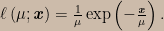
This argument is a straw man caused by a misunderstanding — an unintentional equivocation, if that’s a thing, on the phrase “other portfolios that might have been sent to you but were not”. Now, nothing here turns on the fact that the scenario doesn’t completely specify the distribution of portfolio returns. We are told that the stocks are picked at random, so the portfolio returns are independent and identically distributed random variables; the argument would seem to continue to apply if we specify that portfolio rates of return have some particular known distribution. Mayo tells us that according to a holder of the LP, once x is known we’re not allowed to consider the other chances that the Pickrite method provides for finding an impressive portfolio. Suppose portfolio rates of return are known to have, say, an exponential distribution with unknown mean μ; in that case, the only way I can see to cash out Mayo’s argument in math is to say that she thinks the LP obliges us to use the likelihood function ℓ(μ; x) arising from the exponential density for a single value,

But this is simply wrong. The argument overlooks the fact that the LP doesn’t forbid us from taking the data collection mechanism into account (including mechanisms of missing data) when constructing the likelihood function itself. We’ve been told that we were presented with just the best result from out of k portfolios that were built, so to construct the likelihood we take the probability density for all k rates of return and we integrate out the k – 1 unobserved rates of return that were smaller than the one we do get to see. In statistical jargon, our likelihood function arises from the probability density for the largest order statistic; the general formula for the density of an order statistic can be found here. Assuming as before that rates of return follow an exponential distribution, the correct likelihood arising in this scenario would be

In fact, in this scenario an error statistician would use precisely this probability model to compute “audited” p-values and confidence intervals, and since the parameter being estimated is a scale parameter we would have the standard numerical agreement of frequentist confidence intervals and Bayesian credible intervals (under the usual reference prior for scale parameters).

Kadane might very well ask, “Why are you considering other portfolios that you might have been sent but were not, to reason from the one that you got?” But the portfolios he would be referring to aren’t the other portfolios in the sample that we didn’t get to see — a holder of the LP agrees that those portfolios need to be taken into consideration. The “other portfolios the you might have been sent but were not” are the ones that might have arisen in hypothetical replications of the whole data-generating process, that is, other best portfolios selected out of k of them. Those are the “other portfolios” that likelihood theorists and Bayesians consider irrelevant. (The misunderstanding of the referent of “other portfolios” is the unintentional equivocation.) Of course, an error statistician disagrees that they are irrelevant — they’re implicit in the p-value computation — but this is a separate issue.

So that disposes of the Pickrite scenario and the cherry-picking argument against the LP. The second scenario is attributed to Allan Birnbaum, a statistician who started as a likelihood theorist but later abandoned those views due to the inability of likelihoods to control error probabilities. Here’s how Mayo presents it:

A single observation is made on X, which can take values 1, 2, …, 100. “There are 101 possible distributions conveniently indexed by a parameter θ taking values 0, 1, …, 100″ (ibid.) We are not told what θ is, but there are 101 possible point hypotheses about the value of θ: from 0 to 100. If X is observed to be r, written X = r (r ≠ 0), then the most likely hypothesis is θ = r: in fact, Pr(X = r | θ = r) = 1. By contrast, Pr(X = r | θ = 0) = 0.01. Whatever value r that is observed, hypothesis θ = r is 100 times as likely as is θ = 0. Say you observe X = 50, then H: θ = 50 is 100 times as likely as is θ = 0. So “even if in fact θ = 0, we are certain to find evidence apparently pointing strongly against θ = 0, if we allow comparisons of likelihoods chosen in light of the data” (Cox and Hinkley 1974, p. 52). This does not happen if the test is restricted to two preselected values. In fact, if θ = 0 the probability of a ratio of 100 in favor of the false hypothesis is 0.01.

It’s apparent that this scenario is designed to challenge the views of likelihood theorists more than those of Bayesians. Nevertheless, Mayo writes, “Allan Birnbaum gets the prize for inventing chestnuts that deeply challenge both those who do, and those who do not, hold the Likelihood Principle!” And since Bayesians do hold the LP, let’s see what challenges Birnbaum’s chestnut presents for us Bayesians.

The contention is that if we let the data determine which non-zero θ value to consider then we are certain to find evidence apparently pointing strongly against θ = 0 even if it is in fact the case that θ = 0. That sounds pretty bad!

First we need to say what “evidence pointing against a hypothesis” means for Bayesians. Later in the book Mayo discusses Bayesian epistemology as a school of thought within academic philosophy, including various proposed numerical measures of confirmation. We don’t need to touch on those complications here; for us it will be enough to say that the data provide evidence against a hypothesis when the posterior odds against it are higher than the prior odds.

Because we’re looking at the odds against θ = 0 it is helpful to first decompose the hypothesis space into θ = 0 and its negation θ ≠ 0 and then assign prior probability mass conditional on θ ≠ 0 to the non-zero values, call them θ’, that θ might take. Given such a decomposition, this is the odds form of Bayes’s theorem in this problem:

The ratio on the left is the posterior odds, the first ratio on the right is the prior odds, and the second ratio on the right is the update factor. In the sum in the numerator of the update factor, all of the Pr(X = r | θ = θ’) terms are zero except for the one in which θ’ = r; these terms act as an indicator function selecting just the prior probability for the non-zero θ value corresponding to the observed data value. Since Pr(X = r | θ = 0) = 0.01 we can write

The factor of 100 is the likelihood ratio; perhaps unexpectedly, it can be seen that the likelihood ratio is not only term in the update factor. The Pr(θ = r | θ ≠ 0) term is a funny-looking thing — it’s a prior probability and yet it seems to involve the data. It should be understood to mean “the prior probability, conditional on θ ≠ 0, for the value of θ corresponding to the datum that was later observed”.

Now we can imagine all sorts of background information that might inform our prior probabilities; in this respect the statement of the problem is underspecified. Suppose nevertheless that this is all we are given; then it seems appropriate to specify a uniform conditional prior distribution, Pr(θ = θ’ | θ ≠ 0) = 0.01. Then no matter what value the datum takes, the update factor is identically one; that is, for this prior distribution the evidence in the data is certain to neither cut against nor in favour of θ = 0.

If we have information that justifies a non-uniform conditional prior distribution then for some values of θ the prior will be larger than 0.01; a corresponding datum would result in an update factor greater than one and thus be evidence against θ = 0. But in this situation there must be other values of θ for which the prior is smaller than 0.01, and a corresponding datum would result in an update factor smaller than one and thus be evidence in favour of θ = 0. So contrary to what Cox and Hinkley say holds for likelihood theorists, we Bayesians are never certain of finding evidence against θ = 0 even when it is in fact the case — the closest we get is being certain that the data provide no evidence one way or the other.

I wonder if this chestnut of Birnbaum’s poses any challenge for the severity concept…

How “Severity, part one” got Mayo wrong (and a preview of “Two Severities”)

In the comments to my first post on severity, Professor Mayo noted some apparent and some actual misstatements of her views.To avert misunderstandings, she directed readers to two of her articles, one of which opens by making this distinction:

“Error statistics refers to a standpoint regarding both (1) a general philosophy of science and the roles probability plays in inductive inference, and (2) a cluster of statistical tools, their interpretation, and their justification.”

In Mayo’s writings I see  two interrelated notions of severity corresponding to the two items listed in the quote: (1) an informal severity notion that Mayo uses when discussing philosophy of science and specific scientific investigations, and (2) Mayo’s formalization of severity at the data analysis level.

One of my besetting flaws is a tendency to take a narrow conceptual focus to the detriment of the wider context. In the case of Severity, part one, I think I ended up making claims about severity that were wrong. I was narrowly focused on severity in sense (2) — in fact, on one specific equation within (2) — but used a mish-mash of ideas and terminology drawn from all of my readings of Mayo’s work. When read through a philosophy-of-science lens, the result is a distorted and misstated version of severity in sense (1) .

As a philosopher of science, I’m a rank amateur; I’m not equipped to add anything to the conversation about severity as a philosophy of science. My topic is statistics, not philosophy, and so I want to warn readers against interpreting Severity, part one as a description of Mayo’s philosophy of science; it’s more of a wordy introduction to the formal definition of severity in sense (2).

An adequate analytical approximation to the standard normal CDF

It’s not great, but, as my mother-in-law sometimes says, it’ll do in the dark: