Non-normal bivariate distributions with normal marginal distributions

It’s well known that the ratio of two independent standard normal random variables has a Cauchy distribution. Let’s prove it! Suppose our normal random variables are X and Y. The kernel of the density is

We do this change of variables:

By a happy chance the Jacobian of this transformation is constant and so, with a little harmless disregard for the region of integration, we substitute directly into the joint density function and get

By inspection we can see that we’ve got the joint density of a Cauchy random variable C and, conditional on C, an exponential random variable T with rate (1 + C²)/2. (The kernel of the Cauchy density and the rate parameter of the exponential density are shown explicitly in the second line; in the first line they have effectively cancelled out.) Thus we have shown that the ratio of two independent standard normal random variables is indeed Cauchy.

We can do a little more with this result though. It shows how to generate two independent normal random variates from a Cauchy and an Exponential (and one more random bit) via the following recipe. Generate, independently:

• a Cauchy random variable C,
• a Rademacher random variable S (which takes the value +1 with 50% probability and the value -1 with 50% probability), and
• an Exponential random variable (with rate 1) U.

Set

Independent standard normal random variables aren’t too interesting; this recipe is worth considering because it gives us a way to generate something a lot more fun: three distinct (and very pretty) bivariate distributions, each non-normal but with normal marginal distributions. (Of course, there’s a boring brute force way to make such a distribution: pick any non-Gaussian bivariate copula and push the marginal uniform random variables through the normal quantile function. Yawn.) We’ll do this by making two independent copies of each of the three random variables in our recipe; that is, we’ll have C_i, S_i, and U_i for i ∈ {1,2}. Now we use the i = 1 variables and follow the recipe as above,

And then we mix the indices to create two more marginally normal variables that have a complicated dependence relation to the previous set:

So what kind of distributions did we make? Well, we’ve defined four distinct marginally normal random variables which gives rise to six bivariate distributions. The three interesting distributions are those of (W, X), (W, Y), and (V, Y). The other three pairs fail to spark joy: X and Y are independent standard normal by definition; V and W would be too except I didn’t bother to give them different signs so their joint distribution is only defined in the first and third quadrants; and it turns out that the pair (V, X) just has the same bivariate distribution as (V, Y).

Let’s sample some, uh, samples and see what we get.

And here’s the code, ready to go.

“Baroque possibilities” for constructing SEV in sequential trials

I mentioned in my last post that I had thought up some baroque possibilities for candidate SEV functions in sequential trials. I figure it’s worth writing out exactly what I mean by that. Before I begin, though, I will direct readers to the first 26 slides of this slide deck, especially the plot on slide 6.

As discussed in the slide deck, when you’re designing a two-sided confidence interval procedure you have some freedom to decide, for each value of the true parameter, how much probability mass you will put above (literally above if we’re talking about the plot on slide 6) the upper limit and how much you’ll put below the lower limit. The confidence coverage property only constrains the sum of these two chunks of probability mass.

The kinds of inferences for which the SEV function was designed are one-sided, directional inferences — upper-bounding inferences and lower-bounding inferences — so there’s no arbitrariness to SEV with well-behaved models in fixed sample size designs. Sequential designs introduce multiple thresholds at which alpha can be “spent” so even just for a simple one-sided test there is already an element of arbitrariness that must be eliminated by recourse to an alpha-spending function or an expected sample size minimization or some other principle that eats up the degrees of freedom left over after imposing the Type I error constraint. There is likewise arbitrariness in specifying a one-sided confidence procedure for sequential trials — as with two-sided intervals there are multiple boundaries to specify at each possible parameter value and the confidence coverage constraint only ties up one degree of freedom.

In the last post I asserted that the conditional procedure was an exact confidence procedure. Here’s the math. Let q₄(α, μ) and q₁₀₀(α, μ) be the quantile functions of the conditional distributions:

Then the confidence coverage of the conditional procedure is

The conditional procedure had the difficulty that its inferences could contradict the Type I error rate of the design at the first look. However, we can replace the quantile functions with arbitrary functions as long as they satisfy that same equality for all values of μ and this will also define an exact confidence procedure. The question then becomes what principle/set of constraints/optimization objective can be used to specify a unique choice.

This sort of procedure offers very fine control over alpha-spending at each parameter value, control that is not available via the orderings on the sample space discussed in the last post that that treat values at different sample sizes as directly comparable. But the phrasing of the (S-2) criterion really strongly points to that kind of direct comparison of sample space elements, and Figure 4 of the last post shows that this is a non-starter. So, to defend the SEV approach from my critique it will be necessary to: (i) overhaul (S-2) to allow for the sort of fine control available to fully general confidence procedures, (ii) come up with a principle for uniquely identifying one particular procedure as the SEV procedure, ideally a principle that is in line with severity reasoning as it has been expounded by its proponents up to this point — oh, and (iii) satisfy PRESS, let’s not forget that.

The SEV function just plain doesn’t work

Introduction

I had a different follow-up planned for my last post but I made a discovery (see title) that caused me to change course. Previously I had made the rather weak point that the SEV function had some odd properties that I didn’t think made sense for inference. Mayo’s response (on Twitter) was: “The primary purpose of the SEV requirement is to block inference as poorly warranted, & rigged exes have bad distance measures.” In this post I’ll argue that the SEV function has properties that I don’t think anyone can claim make sense for inference, and I’ll draw out the consequences of affirming the severity rationale in spite of its possession of these undesirable properties.

Here I’ll examine the SEV function in the context of a modification of Mayo’s “water plant accident” example. For the picturesque details you can follow the link; I’ll stick with the math. The model is normal with unknown mean μ and a standard deviation of 10. Here we are interested in testing H₀: μ ≤ 150 vs. H₁: μ > 150. Mayo looks at the test based on the mean of 100 samples, which I will call x̅₁₀₀. My modification is this: we’ll check the mean after collecting 4 samples, x̅₄, and reject the null if it’s greater than some threshold; otherwise we’ll collect the remaining 96 samples and test again using x̅₁₀₀ as our statistic. Which threshold? It hardly matters, but let’s say the threshold for rejection of H₀ and cessation of data collection at n = 4 is at x̅₄ = 165, three standard errors from the null. (This “spends” 0.00135 of whatever Type I error rate we’re willing to tolerate. In Mayo’s example the Type I error rate is set to 0.022, corresponding to a threshold at x̅₁₀₀ = 152, two standard errors from the null; in our case, to compensate for the look at n = 4 the threshold at n = 100 increases a very tiny amount — it’s 152.02. Nothing turns on these details.) I’ll also consider what happens when the design is to collect not 96 but 896 additional samples for a total of 900 before the second look.

This is an early stopping design (a.k.a. group sequential design, adaptive design correction); they’re common in clinical trials where it’s desirable to minimize the number of patients in the event that strong evidence has been observed. Is it a “rigged” example? It sure is. The rigging lies in the fact that in clinical trials the “looks” at the data wouldn’t be as early as this — it generally isn’t worth looking when only 1/25 of the second-look sample size has been observed, much less 1/225. By using this schedule I am deliberately amplifying problems for frequentist inference that already exist in a milder form in more typical trial designs. But we’ve been told that SEV’s primary purpose is to block poorly warranted inferences, and the question we should be asking isn’t “is it rigged?” — it’s whether SEV actually does a reasonable job even in, or perhaps especially in, setups that don’t make a lot of sense. It is, if you will, a severe test of severity reasoning. In any event, I think even a weird design like this ought to be included in the domain of severity reasoning’s application since it’s just twiddling the design parameters of a well-accepted approach.

The postulate on which I’m going to base my argument is this: when early stopping is possible but doesn’t actually occur, the sample mean is consistent for μ and its standard deviation decreases at the usual O(n^-½) rate. So, supposing that we haven’t stopped at the first look, the width of the interval in which the value of μ can be bounded ought in all cases to shrink to zero as we consider designs with larger and larger second-look sample size. This is not a likelihood-based notion — this is based on the conditional distribution of the estimator. When I say SEV doesn’t work, I mean that it fails to adhere to this “Precision RespEcts Sample Size” (PRESS) postulate. If you don’t accept this postulate then I invite you to simulate some data. If you still don’t accept this postulate then my argument that SEV doesn’t work may not be convincing to you, but you’ll find that you have to take on board some troubling consequences nevertheless.

(Just to set expectations: the rest of this post is about ten times longer than this introduction; there are equations and plots.)

Challenges to the Likelihood Principle in Mayo’s new book

I’ve been reading Mayo’s recent book, Statistical Inference as Severe Testing, and I’ve arrived at the chapter in which she offers criticisms of the Likelihood Principle (LP) (recall that the LP says that the data should enter into the inference only through the likelihood function). In contrast, Mayo’s severity approach directs us to examine a procedure’s capacity to detect errors; in practice this means computing, post-data, how frequently a procedure’s actual conclusion could have been reached in error in hypothetical repetitions. Data enters into the inference as part of a sampling distribution calculation, so severity and the LP are incompatible. In this post I’ll examine two of the scenarios Mayo presents while criticizing the LP; I aim to demonstrate that in the first scenario the criticism Mayo offers is founded on a technical error, and in the second scenario the criticism Mayo offers may bite against likelihood theorists but is toothless for Bayesians.

The first scenario concerns an investment fund that deceptively advertises portfolio picks made by the “Pickrite method”:

[Jay] Kadane[, a prominent Bayesian,] is emphasizing that Bayesian inference is conditional on the particular outcome. So once x is known and fixed, other possible outcomes that could have occurred but didn’t are irrelevant. Recall finding that Pickrite’s procedure was to build k different portfolios [with a random selection of stocks] and report just the one that did best. It’s as if Kadane is asking: “Why are you considering other portfolios that you might have been sent but were not, to reason from the one that you got?” Your answer is: “Because that’s how I figure out whether your boast about Pickrite is warranted.” With the “search through k portfolios” procedure, the possible outcomes are the success rates of the k different attempted portfolios, each with its own null hypothesis. The actual or “audited” P-value is rather high, so the severity for H: Pickrite has a reliable strategy, is low (1 – p). For the holder of the LP to say that, once x is known, we’re not allowed to consider the other chances that they gave themselves to find an impressive portfolio, is to put the kibosh on a crucial way to scrutinize the testing process.

This argument is a straw man caused by a misunderstanding — an unintentional equivocation, if that’s a thing, on the phrase “other portfolios that might have been sent to you but were not”. Now, nothing here turns on the fact that the scenario doesn’t completely specify the distribution of portfolio returns. We are told that the stocks are picked at random, so the portfolio returns are independent and identically distributed random variables; the argument would seem to continue to apply if we specify that portfolio rates of return have some particular known distribution. Mayo tells us that according to a holder of the LP, once x is known we’re not allowed to consider the other chances that the Pickrite method provides for finding an impressive portfolio. Suppose portfolio rates of return are known to have, say, an exponential distribution with unknown mean μ; in that case, the only way I can see to cash out Mayo’s argument in math is to say that she thinks the LP obliges us to use the likelihood function ℓ(μ; x) arising from the exponential density for a single value,

But this is simply wrong. The argument overlooks the fact that the LP doesn’t forbid us from taking the data collection mechanism into account (including mechanisms of missing data) when constructing the likelihood function itself. We’ve been told that we were presented with just the best result from out of k portfolios that were built, so to construct the likelihood we take the probability density for all k rates of return and we integrate out the k – 1 unobserved rates of return that were smaller than the one we do get to see. In statistical jargon, our likelihood function arises from the probability density for the largest order statistic; the general formula for the density of an order statistic can be found here. Assuming as before that rates of return follow an exponential distribution, the correct likelihood arising in this scenario would be

In fact, in this scenario an error statistician would use precisely this probability model to compute “audited” p-values and confidence intervals, and since the parameter being estimated is a scale parameter we would have the standard numerical agreement of frequentist confidence intervals and Bayesian credible intervals (under the usual reference prior for scale parameters).

Kadane might very well ask, “Why are you considering other portfolios that you might have been sent but were not, to reason from the one that you got?” But the portfolios he would be referring to aren’t the other portfolios in the sample that we didn’t get to see — a holder of the LP agrees that those portfolios need to be taken into consideration. The “other portfolios the you might have been sent but were not” are the ones that might have arisen in hypothetical replications of the whole data-generating process, that is, other best portfolios selected out of k of them. Those are the “other portfolios” that likelihood theorists and Bayesians consider irrelevant. (The misunderstanding of the referent of “other portfolios” is the unintentional equivocation.) Of course, an error statistician disagrees that they are irrelevant — they’re implicit in the p-value computation — but this is a separate issue.

So that disposes of the Pickrite scenario and the cherry-picking argument against the LP. The second scenario is attributed to Allan Birnbaum, a statistician who started as a likelihood theorist but later abandoned those views due to the inability of likelihoods to control error probabilities. Here’s how Mayo presents it:

A single observation is made on X, which can take values 1, 2, …, 100. “There are 101 possible distributions conveniently indexed by a parameter θ taking values 0, 1, …, 100″ (ibid.) We are not told what θ is, but there are 101 possible point hypotheses about the value of θ: from 0 to 100. If X is observed to be r, written X = r (r ≠ 0), then the most likely hypothesis is θ = r: in fact, Pr(X = r | θ = r) = 1. By contrast, Pr(X = r | θ = 0) = 0.01. Whatever value r that is observed, hypothesis θ = r is 100 times as likely as is θ = 0. Say you observe X = 50, then H: θ = 50 is 100 times as likely as is θ = 0. So “even if in fact θ = 0, we are certain to find evidence apparently pointing strongly against θ = 0, if we allow comparisons of likelihoods chosen in light of the data” (Cox and Hinkley 1974, p. 52). This does not happen if the test is restricted to two preselected values. In fact, if θ = 0 the probability of a ratio of 100 in favor of the false hypothesis is 0.01.

It’s apparent that this scenario is designed to challenge the views of likelihood theorists more than those of Bayesians. Nevertheless, Mayo writes, “Allan Birnbaum gets the prize for inventing chestnuts that deeply challenge both those who do, and those who do not, hold the Likelihood Principle!” And since Bayesians do hold the LP, let’s see what challenges Birnbaum’s chestnut presents for us Bayesians.

The contention is that if we let the data determine which non-zero θ value to consider then we are certain to find evidence apparently pointing strongly against θ = 0 even if it is in fact the case that θ = 0. That sounds pretty bad!

First we need to say what “evidence pointing against a hypothesis” means for Bayesians. Later in the book Mayo discusses Bayesian epistemology as a school of thought within academic philosophy, including various proposed numerical measures of confirmation. We don’t need to touch on those complications here; for us it will be enough to say that the data provide evidence against a hypothesis when the posterior odds against it are higher than the prior odds.

Because we’re looking at the odds against θ = 0 it is helpful to first decompose the hypothesis space into θ = 0 and its negation θ ≠ 0 and then assign prior probability mass conditional on θ ≠ 0 to the non-zero values, call them θ’, that θ might take. Given such a decomposition, this is the odds form of Bayes’s theorem in this problem:

The ratio on the left is the posterior odds, the first ratio on the right is the prior odds, and the second ratio on the right is the update factor. In the sum in the numerator of the update factor, all of the Pr(X = r | θ = θ’) terms are zero except for the one in which θ’ = r; these terms act as an indicator function selecting just the prior probability for the non-zero θ value corresponding to the observed data value. Since Pr(X = r | θ = 0) = 0.01 we can write

The factor of 100 is the likelihood ratio; perhaps unexpectedly, it can be seen that the likelihood ratio is not only term in the update factor. The Pr(θ = r | θ ≠ 0) term is a funny-looking thing — it’s a prior probability and yet it seems to involve the data. It should be understood to mean “the prior probability, conditional on θ ≠ 0, for the value of θ corresponding to the datum that was later observed”.

Now we can imagine all sorts of background information that might inform our prior probabilities; in this respect the statement of the problem is underspecified. Suppose nevertheless that this is all we are given; then it seems appropriate to specify a uniform conditional prior distribution, Pr(θ = θ’ | θ ≠ 0) = 0.01. Then no matter what value the datum takes, the update factor is identically one; that is, for this prior distribution the evidence in the data is certain to neither cut against nor in favour of θ = 0.

If we have information that justifies a non-uniform conditional prior distribution then for some values of θ the prior will be larger than 0.01; a corresponding datum would result in an update factor greater than one and thus be evidence against θ = 0. But in this situation there must be other values of θ for which the prior is smaller than 0.01, and a corresponding datum would result in an update factor smaller than one and thus be evidence in favour of θ = 0. So contrary to what Cox and Hinkley say holds for likelihood theorists, we Bayesians are never certain of finding evidence against θ = 0 even when it is in fact the case — the closest we get is being certain that the data provide no evidence one way or the other.

I wonder if this chestnut of Birnbaum’s poses any challenge for the severity concept…

Everything I never got around to writing about severity

The first post on this blog described my blogging agenda. It was pinned to the top of the blog but it’s badly out of date so I’ve unpinned it. When I left off, I was about half way though my explanation of severity and I was about to embark on a description of what Mayo calls “howlers” – calumnies cast upon the classical tools of frequentist statistics that are addressed by the severity concept. The severity concept and its formal mathematical incarnation, the SEV function, are explained in Mayo and Spanos’s 2011 article Error Statistics, as are the ways in which the SEV function addresses typical criticisms (which are helpfully written in bold font in numbered and center-justified boxes, but SEV isn’t introduced until howler #2).

I recommend that people who want to really understand the severity argument read the above-linked paper, but for completeness’s sake let’s have a look at how the SEV function formalizes severity arguments. (Since I’ll be discussing both frequentist and Bayesian calculations I’ll use the notation Fr ( · ; · ) for frequency distributions and Pl ( · | · ) for plausibility distributions.) The examples I’ve seen typically involve nice models and location parameters, so let’s consider an irregular model with a scale parameter. Consider a univariate uniform distribution with unknown support; suppose that the number of data points, n, is at least two and we aim to assess the warrant for claims about the width of the support, call it ∆, using the difference between the largest and smallest data values, D = X_max – X_min, as our test statistic. (This model is “irregular” in that the support of the test statistic’s sampling distribution depends on the parameter.) Starting from the joint distribution of the order statistics of the uniform distribution one can show that D is a pivotal statistic satisfying

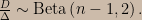
Severity reasoning works like this: we aim to rule out a particular way that some claim could be wrong, thereby avoiding one way of being in error in asserting the claim. The way we do that is by carrying out a test that would frequently detect such an error if the claim were in fact wrong in that particular way. We attach the error detection frequency to the claim and say that the claim has passed a severe test for the presence of the error; the error detection frequency quantifies just how severe the test was.

To cash this out in the form of a SEV function we need a notion of accordance between the test statistic and the statistical hypothesis being tested. In our case, higher observed values of D accord with higher hypothesized values of ∆ (and in fact, values of ∆ smaller than the observed value of D are strictly ruled out). SEV is a function with a subjunctive mood; we don’t necessarily carry out any particular test but instead look at all the tests we might have carried out. So: if we were to claim that ∆ > δ when ∆ ≤ δ was true then we’d have committed an error. Smaller observed values of D are less in accord with larger values of ∆, so we could have tested for the presence of the error by declaring it to be present if the observed value of D were smaller than some threshold d. Now, there are lots of possible thresholds d and also lots of ways that the claim “∆ > δ” could be wrong – one way for each value of ∆ smaller than δ – but we can finesse these issues by considering the worst possible case. In the worst case the test is just barely passed, that is, the observed value of D is on the test’s threshold, and ∆ takes the value that minimizes the frequency of error detection and yet still satisfies ∆ ≤ δ. (Mayo does more work to justify all of this than I’m going to do here.) Thus the severity of the test that the claim “∆ > δ” would have passed is the worst-case frequency of declaring the error to be present supposing that to actually be the case:

in which D is (still) a random variable and d is the value of D that was actually observed in the data at hand.

In every example of a SEV calculation I’ve seen, the minimum occurs right on the boundary — in this case, at ∆ = δ. It’s not clear to me if Mayo would insist that the SEV function can only be sensibly defined for models in which the minimum is at the boundary; that restriction seems implicit in some of the things she’s written about accordance of test statistics with parameter values. In any event it holds in this model, so we can write

What this says is that to calculate the SEV function for this model we stick (d / δ) into the cdf for the Beta (n – 1, 2) distribution and allow δ to vary. I’ve written a little web app to allow readers to explore the meaning of this equation.

As part of my blogging agenda I had planned to find examples of prominent Bayesians asserting Mayo’s howlers. At one point Mayo expressed disbelief to me that I would call out individuals by name as I demonstrated how the SEV function addressed their criticism, but this would have been easier for me than she thought. The reason is that in all of the examples of formal SEV calculations that I have ever seen (including the one I just did above), it’s been applied to univariate location or scale parameter problems in which the SEV calculation produces exactly the same numbers as a Bayesian analysis (using the commonly-accepted default/non-informative/objective prior, i.e., uniform for location parameters and/or for the logarithm of scale parameters; this SEV calculator web app for the normal distribution mean serves equally well as a Bayesian posterior calculator under those priors). So I wasn’t too concerned about ruffling feathers – because I’m no one of consequence, but also because a critique that goes “criticisms of frequentism are unfair because frequentists have figured out this Bayesian-posterior-looking thing” isn’t the sort of thing any Bayesian is going to find particularly cutting, no matter what argument is adduced to justify the frequentist posterior analogue. In any event, at this remove I find I lack the motivation to actually go and track down an instance of a Bayesian issuing each of the howlers, so if you are one such and you’ve failed to grapple with Mayo’s severity argument – consider yourself chided! (Although I can’t be bothered to find quotes I can name a couple of names off the top of my head: Jay Kadane and William Briggs.)

Because of this identity of numerical output in the two approaches I found it hard to say whether the SEV functions computed and plotted in Mayo and Spanos’s article and in my web app illustrate the severity argument in a way that actually supports it or if they’re just lending it an appearance of reasonability because, through a mathematical coincidence, they happens to line up with default Bayesian analyses. Or, perhaps default Bayesian analyses seem to give reasonable numbers because, through a mathematical coincidence, they happen to line up with SEV – a form of what some critics of Bayes have called “frequentist pursuit”. To help resolve this ambiguity I sought to create an intuition pump: an easy-to-analyze statistical model that could be subjected to extreme conditions in which intuition would strongly suggest what sorts of conclusions were reasonable. The outputs of the formal statistical methods — the SEV function on the one hand and a Bayesian posterior on the other — could be measured relative to these intuitions. Of course, sometimes the point of carrying out a formal analysis is to educate one’s intuition, as in the birthday problem; but in other cases one’s intuition acts to demonstrate that the formalization isn’t doing the work one intended it to do, as in the case of the integrated information theory of consciousness. (The latter link has a discussion of “paradigm cases” that is quite pertinent to my present topic.)

When I first started blogging about severity the idea I had in mind for this intuition pump was to apply an optional stopping data collection design to the usual normal distribution with known variance and unknown mean. Either one or two data points would be observed, with the second data point observed only if the first one was within some region where it would be desirable to gather more information. This kind of optional stopping design induces the same likelihood function (up to proportionality) as a fixed sample size design, but the alteration of the sample space gives rise to very different frequency properties, and this guarantees that (unlike in the fixed sample sized design) the SEV function and the Bayesian posterior will not agree in general.

Now, the computation of a SEV function demands a test procedure that gives a rejection region for any Type I error rate and any one-sided alternative hypothesis; this is because to calculate SEV we need to be able to run the test procedure backward and figure out for each possible one-sided alternative hypothesis what Type I error rate would have given rise to a rejection region with the observed value of the test statistic right on the boundary. (If that seemed complicated, it’s because it is.) In the optional stopping design the test procedure would involve two rejection regions, one for each possible sample size, and a collect-more-data region; given these extra degrees of freedom in specifying the test I found myself struggling to define a procedure that I felt could not be objected to – in particular, I couldn’t handle the math needed to find a uniformly most powerful test (if one even exists in this setup). The usual tool for proving the existence of uniformly powerful tests, the Karlin-Rubin theorem, does not apply to the very weird sample space that arises in the optional stopping design – the dimensionality of the sample space is itself a random variable. But as I worked with the model I realized that optional stopping wasn’t the only way to alter the sample space to drive a wedge between the SEV function and the Bayesian posterior. When I examined the first stage of the optional stopping design in which the collect-more-data region creates a gap in the sample space, I realized that chopping out a chunk of the sample space and just forgetting about the second data point would be enough to force the two formal statistical methods to disagree.

An instance of such a model was described in my most recent post: a normal distribution with unknown μ in ℝ and unit σ and a gap in the sample space between -1 and 3, yielding the probability density

As previously mentioned, the formalization of severity involves some kind of notion of accordance between test statistic values and parameter values. For the gapped normal distribution the Karlin-Rubin theorem applies directly: a uniformly most powerful test exists and it’s a threshold test, just as in the ordinary normal model. So it seems reasonable to say that larger values of x accord with larger values of μ even with the gap in the sample space, and the SEV function is constructed for the gapped normal model just as it would be for the ordinary normal model:

It’s interesting to note that frequentist analyses such as a p-value or the SEV function will yield the same result for x = -1 and x = 3. In both these cases, for example,

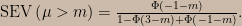
This is because the data enter into the inference through tail areas of the sampling probability density, and those tail areas are the same whether the interval of integration has its edge at x = -1 or x = 3.

The Bayesian posterior distribution, on the other hand, involves integration over the parameter space rather than the sample space. Assuming a uniform prior for μ, the posterior distribution is

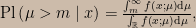
which does not have an analytical solution. We can see right away that the Bayesian posterior will not yield the same result when x = -1 as it does when x = 3 because the data enter into the inference through the likelihood function, and x = -1 induces a different likelihood function than x = 3.

But what about that uniform prior? Does a prior exist that will enable “frequentist pursuit” and bring the Bayesian analysis and the SEV function back into alignment? To answer this question, consider the absolute value of the derivative of the SEV function with respect to m. This is the “SEV density”, the function that one would integrate over the parameter space to recover SEV. I leave it as an exercise for the reader to verify that this function cannot be written as (proportional to) the product of the likelihood function and a data-independent prior density.

So! I have fulfilled the promise I made in my blogging agenda to specify a simple model in which the two approaches, operating on the exact same information, must disagree. It isn’t the model I originally thought I’d have – it’s even simpler and easier to analyze. The last item on the agenda is to subject the model to extreme conditions so as to magnify the differences between the SEV function and the Bayesian approach. This web app can be used to explore the two approaches.

The default setting of the web app shows a comparison I find very striking. In this scenario x = -1 and Pl(μ > 0 | x) = 0.52. (Nothing here turns on the observed value being right on the boundary – we could imagine it to be slightly below the boundary, say x = -1.01, and the change in the scenario would be correspondingly small.) This reflects the fact that x = -1 induces a likelihood function that has a fairly broad peak with a maximum near μ = 0. That is, the probability of landing in a vanishingly small neighbourhood of the value of x we actually observed is high in a relative sense for values of μ in a broad range that extends on both sides of μ = 0; when we normalize and integrate over μ > 0 we find that we’ve captured about half of the posterior plausibility mass. On the other hand, SEV(μ > 0) = 0.99. The SEV function is telling us that if μ > 0 were false then we would very frequently – at least 99 times out of 100 – have observed values of x that accord less well with μ > 0 than the one we have in hand. But wait – severity isn’t just about the subjunctive test result; it also requires that the data “accords with” the claim being made in an absolute sense. If μ = 1 then x = -1 is a median point of the sampling distribution, so I judge that x = -1 does indeed accord with μ > 0.

I personally find my intuition rebels against the idea that “μ > 0″ is a well-warranted claim in light of x = -1; it also rebels at the notion than x = -1 and x = 3 provide equally good warrant for the claim that μ > 0. In the end, I strictly do not care about regions of the sample space far away from the observed data. In fact, this is the reason that I stopped blogging about this – about four years ago I took one look at that plot and felt my interest in (and motivation for writing about) the severity concept drain away. Since then, this whole thing has been weighing down my mind; the only reason I’ve managed to muster the motivation to finally get it out there is because I was playing around with Shiny apps recently – they’ve got a lot better since the last time I did so, which was also about four years ago – and started thinking about the visualizations I could make to illustrate these ideas.

A statistical model and a question about inference

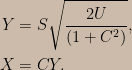
Consider a normal distribution with unknown μ and unit variance, but with a twist: the sample space has a gap in it between -1 and 3. Accounting for the gap, the resulting probability density becomes:

In this model μ is not quite a location parameter; when it’s far from the gap the density is effectively a normal centered at μ but when it’s close to the gap its shape is distorted. It becomes a half-normal at the gap boundary and then something like an extra-shallow exponential (log-quadratic instead of log-linear like an actual exponential) as μ moves toward the center of the gap. At μ = 1 the probability mass flips from one side of the gap to the other. Here’s a little web app in which you can play around with this statistical model (don’t neglect the play button under the slider on the right hand side).

Now the question; I ask my readers to report their gut reaction in addition to any more considered conclusions in comments.

Suppose μ is unknown and the data is a single observation x. Consider two scenarios:

1. x = -1 (the left boundary)
2. x = 3 (the right boundary)

For the sake of concreteness suppose our interest is in μ ≤ 0 vs. μ > 0. Should it make a difference to our inference whether we’re in scenario (i) or scenario (ii)?

Laurie Davies and betting on adequacy

About a year and a half ago, I read P. L. Davies’s interesting paper Approximating Data. There was one passage I read that struck me as unusually wrong-headed (pg 195):

The Dutch book argument in turn relies on a concept of truth. Often framed in terms of bets on a horse-race, it relies on there only being one winner, which is the case for the overwhelming majority of horse races. The Dutch book argument shows that the odds, when converted to probabilities, must sum to 1 to avoid arbitrage possibilities… If we transfer this to statistics then we have different distributions indexed by a parameter. Based on the idea of truth, only one of these can be true, just as only one horse can win, and the same Dutch book argument shows that the odds must add to 1. In other words the prior must be a probability distribution. We note that in reality none of the offered distributions will be the truth, but due to the non-callability of Bayesian bets this is not considered to be a problem. Suppose we replace the question as whether a distribution represents the truth by the question as to whether it is a good approximation. Suppose that we bet, for example, that the N(0, 1) distribution is an adequate approximation for the data. We quote odds for this bet, the computer programme is run, and we either win or lose. If we quote odds of 5:1 then we will probably quote the same, or very similar, odds for the N(10⁻⁶, 1) distribution, as for the N(0, 1+10⁻¹⁰) distribution and so forth. It becomes clear that these odds are not representable by a probability distribution: only one distribution can be the ‘true’ but many can be adequate approximations.

I always meant to write something about how this line of argument goes wrong, but it wasn’t a high priority. But recently Davies reiterated this argument in a comment on Professor Mayo’s blog:

You define adequacy in a precise manner, a computer programme., there [sic] are many examples in my book. The inputs are the data and the model, the output yes or no. You place your bets beforehand, run the programme and win or lose your bet. The bets are realizable. If you bet 50-50 on the N(0,1) being an adequate model, you will no doubt bet about 50-50 on the N(10^-20,1) also being an adequate model. Your bets are not expressible by a probability measure. The sum of the odds will generally be zero or infinity. …

I tried to reply in the comment thread, but WordPress ate my attempts, so: a blog post!

I have to wonder if Professor Davies asked even one Bayesian to evaluate this argument before he published it. (In comments, Davies replies: I have been stating the argument for about 20 years now. Many Bayesians have heard my talks but so the only response I have had was by one in Lancaster who told me he had never heard the argument before and that was it.) Let M be the set of statistical models under consideration. It’s true that if I bet 50-50 on N(0,1) being an adequate model, I will no doubt bet very close to 50-50 on N(10^-20, 1) also being an adequate model. Does this mean that “these odds are not representable by a probability distribution”? Not at all — we just need to get the sample space right. In this setup the appropriate sample space for a probability triple is the powerset of M, because exactly one of the members of the powerset of M will be realized when the data become known.

For example, suppose that M = {N(0,1), N(10^-20, 1), N(10,1)}; then there are eight conceivable outcomes — one for each possible combination of adequacy indications — that could occur once the data become known. We can encode this sample space using the binary expansion of the numbers from 0 to 7, with each digit of the binary expansion of the integer interpreted as an indicator variable for the statistical adequacy of one of the models in M. Let the leftmost bit refer to N(0,1), the center bit refer to N(10^-20, 1), and the rightmost bit refer to N(10,1). Here’s a probability measure that serves as a counterexample to the claim that “[the 50-50] bets are not expressible by a probability measure”:

Pr(001) = Pr(110) = 0.5,

Pr(000) = Pr(100) = Pr(101) = Pr(011) = Pr(010) = Pr(111) = 0.

(This is an abuse of notation, since the Pr() function takes events, that is, sets of outcomes, and not raw outcomes.) The events Davies considers are “N(0,1) [is] an adequate model”, which is the set {100, 101, 110, 111}, and “N(10^-20,1) [is] an adequate model”, which is the set {010, 011, 110, 111}; it is trivial to see that both these events are 50-50.

Now obviously when M is uncountably infinite it’s not so easy to write down probability measures on sigma-algebras of the powerset of M. Still, that scenario is not particularly difficult for a Bayesian to handle: if the statistical adequacy function is measurable, a prior or posterior predictive probability measure automatically induces a pushforward probability measure on any sigma-algebra of the powerset of M. In fact, this is precisely the approach taken in the (rather small) Bayesian literature on assessing statistical adequacy; see for example A nonparametric assessment of model adequacy based on Kullback-Leibler divergence. These sorts of papers typically treat statistical adequacy as a continuous quantity, but all it would take to turn it into a Davies-style yes-no Boolean variable would be to dichotomize the continuous quantity at some threshold.

(A digression. To me, using a Bayesian nonparametric posterior distribution to assess the adequacy of a parametric model seems a bit pointless — if you have the posterior already, of what possible use is the parametric model? Actually, there is one use that I can think of, but I was saving it to write a paper about… Oh what the heck. I’m told (by Andrew Gelman, who should know!) that in social science it’s notorious that every variable is correlated with every other variable, at least a little bit. I imagine that this makes Pearl-style causal inference a big pain — all of the causal graphs would end up totally connected, or close to. I think there may be a role for Bayesian causal graph adequacy assessment; the causal model adequacy function would quantify the loss incurred by ignoring some edges in the highly-connected causal graph. I think this approach could facilitate communication between causal inference experts, subject matter experts, and policymakers.)

This post’s title was originally more tendentious and insulting. As Professor Davies has graciously suggested that his future work might include a reference to this post, I think it only polite that I change the title to something less argumentative.

How “Severity, part one” got Mayo wrong (and a preview of “Two Severities”)

In the comments to my first post on severity, Professor Mayo noted some apparent and some actual misstatements of her views.To avert misunderstandings, she directed readers to two of her articles, one of which opens by making this distinction:

“Error statistics refers to a standpoint regarding both (1) a general philosophy of science and the roles probability plays in inductive inference, and (2) a cluster of statistical tools, their interpretation, and their justification.”

In Mayo’s writings I see  two interrelated notions of severity corresponding to the two items listed in the quote: (1) an informal severity notion that Mayo uses when discussing philosophy of science and specific scientific investigations, and (2) Mayo’s formalization of severity at the data analysis level.

One of my besetting flaws is a tendency to take a narrow conceptual focus to the detriment of the wider context. In the case of Severity, part one, I think I ended up making claims about severity that were wrong. I was narrowly focused on severity in sense (2) — in fact, on one specific equation within (2) — but used a mish-mash of ideas and terminology drawn from all of my readings of Mayo’s work. When read through a philosophy-of-science lens, the result is a distorted and misstated version of severity in sense (1) .

As a philosopher of science, I’m a rank amateur; I’m not equipped to add anything to the conversation about severity as a philosophy of science. My topic is statistics, not philosophy, and so I want to warn readers against interpreting Severity, part one as a description of Mayo’s philosophy of science; it’s more of a wordy introduction to the formal definition of severity in sense (2).

When does Bayesian inference shatter?

In the spring of last year, a paper with the title Bayesian Brittleness: Why no Bayesian model is “good enough”  was put on the arXiv. The authors (Houman Owhadi, Clint Scovel, Tim Sullivan, henceforth OSS) later posted a followup entitled When Bayesian inference shatters. When published, this work was commented on in a number of stats blogs I follow, including Xian’s Og and Error Statistics Philosophy. Christian Hennig wrote up this nice nickel summary:

One of the author’s results (if I could nominate one as the most important, I’d choose this one) says that if you replace your model by another one which is in an arbitrarily close neighborhood (according to the [Prokhorov] metric discussed above), the posterior expectation could be as far away as you want. Which, if you choose the right metric, means that you replace your sampling model by another one out of which typical samples *look the same*, and which therefore can be seen as as appropriate for the situation as the original one.

Note that the result is primarily about a change in the sampling model, not the prior, although it is a bit more complex than that because if you change the sampling model, you need to adapt the prior, too, which is appropriately taken into account by the authors as far as I can see.

My own reaction was rather less impressed; I tossed off,

Conclusion: Don’t define “closeness” using the TV [that is, total variation] metric or matching a finite number of moments. Use KL divergence instead.

In response to a a request by Mayo, OSS wrote up a “plain jane” explanation which was posted on Error Statistics Philosophy a couple of weeks later. It confirmed Christian’s summary:

So the brittleness theorems state that for any Bayesian model there is a second one, nearly indistinguishable from the first, achieving any desired posterior value within the deterministic range of the quantity of interest.

That sounds pretty terrible!

—

This issue came up for discussion in the comments of an Error Statistics Philosophy post in late December.

MAYO: Larry: Do you know anything about current reactions to, status of, the results by Houman Owhadi, Clint Scovel and Tim Sullivan? Are they deemed relevant for practice? (I heard some people downplay the results as not of practical concern.)

LARRY: I am not aware of significant rebuttals.

COREY: I have a vague idea that any rebuttal will basically assert that the distance these authors use is too non-discriminating in some sense, so Bayes fails to distinguish “nice” distributions from nearby (according to the distance) “nasty” ones. My intuition is that these results won’t hold for relative entropy, but I don’t have the knowledge and training to develop this idea — you’d need someone like John Baez for that.

OWHADI (the O in OSS): Well, one should define what one means by “nice” and “nasty” (and preferably without invoking circular arguments).

Also, it would seem to me that the statement that TV and Prokhorov cannot be used (or are not relevant) in “classical” Bayes is a powerful result in itself. Indeed TV has not only been used in many parts of statistics but it has also been called the testing metric by Le Cam for a good reason: i.e. (writing n the number of samples), Le Cam’s Lemma state that
1) For any n, if TV is close enough (as a function of n) all tests are bad.
2) Given any TV distance, with enough sample data there exists a good test.

Now concerning using closeness in Kullback–Leibler (KL) divergence rather than Prokhorov or TV, observe that (as noted in our original post) closeness in KL divergence is not something you can test with discrete data, but you can test closeness in TV or Prokhorov. In other words the statement “if the true distribution and my model are close in KL then classical Bayes behaves nicely” can be understood as “if I am given this infinite amount of information then my Bayesian estimation is good” which is precisely one issue/concern raised by our paper (brittleness under “finite” information).

Note also that, the assumption of closeness in KL divergence requires the non-singularity of the data generating distribution with respect to the Bayesian model (which could be a very strong assumption if you are trying to certify the safety of a critical system and results like the Feldman–Hajek Theorem tell us that “most” pairs of measures are mutually singular in the now popular context of stochastic PDEs).

In preparing a reply to Owhadi, I discovered a comment written by Dave Higdon on Xian’s Og a few days after OSS’s “plain jane” summary went up on Error Statistics Philosophy. He described the situation in concrete terms; this clarified for me just what it is that OSS’s brittleness theorems demonstrate. (Christian Hennig saw the issue too, but I couldn’t follow what he was saying without the example Higdon gave. And OSS are perfectly aware of it too — this post represents me catching up with the more knowledgeable folks.)

Suppose we judge a system safe provided that the probability that the random variable X exceeds 10 is very low. We assume that X has a Gaussian distribution with known variance 1 and unknown mean μ, the prior for which is

This prior doesn’t encode a strong opinion about the prior predictive probability of the event X > 10 (i.e., disaster).

Next, we learn about the safety of the system by observing a realization of X, and it turns out that the datum x is smaller than 7 and the posterior predictive probability of disaster is negligible. Good news, right?

OSS say, not so fast! They ask: suppose that our model is misspecified, and the true model is “nearby” in Prokhorov or TV metric. They show that for any datum that we can observe, the set of all nearby models includes a model that predicts disaster.

What kinds of model misspecifications do the Prokhorov and TV metrics capture? Suppose that the data space has been discretized to precision 2ϵ, and consider the set of models in which, for each possible observable datum x₀, the probability density is

in which χ(.) is the indicator function. For any specific value of μ, all of the models in the above set are within a small ball centered on the Gaussian model, where “small” is measured by either the Prokhorov or  TV metric. (How small depends on ϵ.)  Each model embodies an implication of the form:

by taking the contrapositive, we see that this is equivalent to:

Each of these “nearby” models basically modifies the Gaussian model to enable one specific possible datum to be a certain indicator of disaster. Thus, no matter which datum we actually end up observing, there is a “nearby” model for which both (i) typical samples are basically indistinguishable from typical samples under our assumed Gaussian model, and yet (ii) the realized datum has caused that “nearby” model, like Chicken Little, to squawk that the sky is falling.

OSS have proved a very general version of the above phenomenon: under the (weak) conditions they assume, for any given data set that we can observe, the set of all models “near” the posterior distribution contains a model that, upon observation of the realized data, goes into (the statistical model equivalent of) spasms of pants-shitting terror.

There’s nothing special to Bayes here; in particular, all of the talk about the asymptotic testability of TV- and/or Prokhorov-distinct distributions is a red herring. The OSS procedure stymies learning about the system of interest because the model misspecification set is specifically constructed to allow any possible data set to be totally misleading under the assumed model. Seen in this light, OSS’s choice of article titles is rather tendentious, don’t you think? If tendentious titles are the order of the day, perhaps the first one could be called As flies to wanton boys are we to th’ gods: Why no statistical model whatsoever is “good enough”  and the second one could be called Prokhorov and total variation neighborhoods and paranoid psychotic breaks with reality.

An adequate analytical approximation to the standard normal CDF

It’s not great, but, as my mother-in-law sometimes says, it’ll do in the dark: